Independent t-test
Plotting the data is a good way to get a feel for differences between groups, but statistics can provide us with two more pieces of information: a confidence interval for the difference between means and a measure of the probability that an effect is due to chance (statistical significance). We will use an independent samples t-test to do our analysis.
Independent Samples t-test
To access the test, select t-test on the list of analyses across the top bar on Jamovi. You should see this:
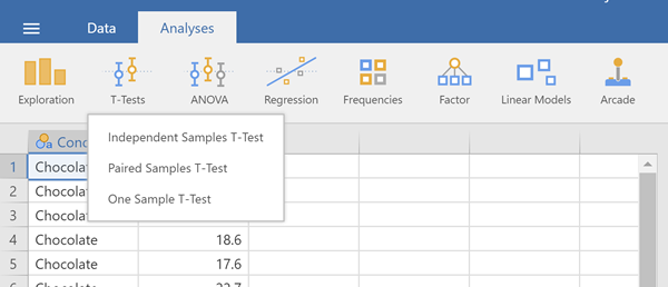
It is good to see that there are multiple types of t-tests. In this case we are doing an independent t-test. Why? When might yiou do an pair samples (or dependent) t-test? In the dialog that appears, put "Tip_Percentage" in the "Dependent Variables" window and "Condittion" into the "Grouping Variable" window as shown below.
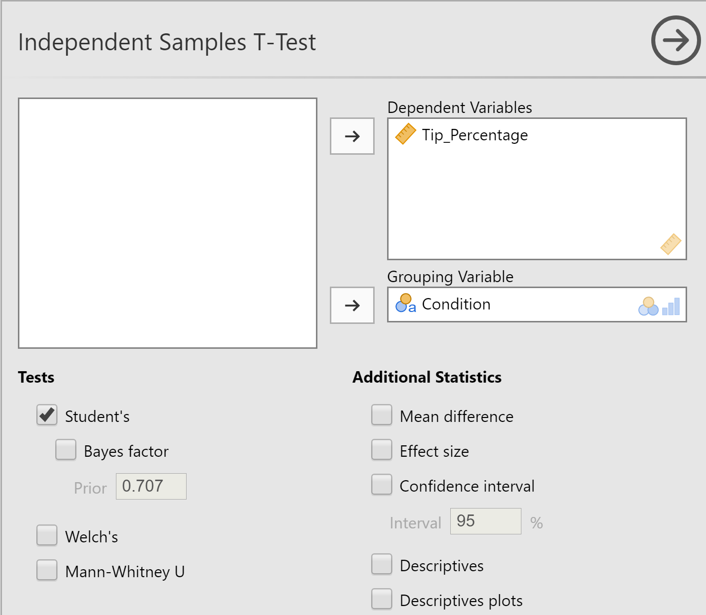
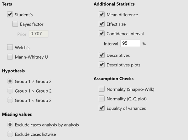
There are a lot of additional options on the analysis. In the checkboxes below where you entered the variables for analsys, select, under Additional Statistics "Mean Difference," "Effect Size," "Confidence Interval," "Descriptives", and "Descriptive Plots". Under Assumption Checks, select "Equality of Variances." While we are notice under Hypothesis that we are selected a two-tailed t-test where all we are hypothesizing is that Mean 1 does not equal Mean 2.
Output
Let us now look at the output window and see what we get from our t-test.
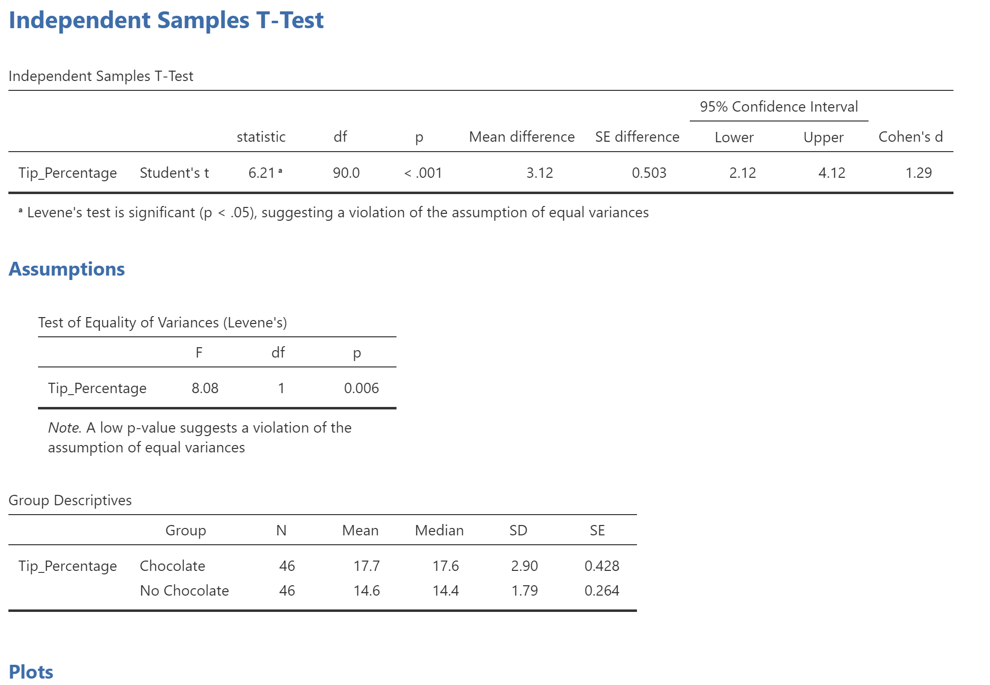
First, let us look at the descriptive statistics on each level of your independent variable: You can find it on th eoutput window below the Assumptions test and right above the Plots.
The mean for the Chocolate condition is 17.74, and for No Chocolate it is 14.62. As we saw in the boxplot, the dispersion (measured by standard deviation) is greater in the Chocolate condition than the No Chocolate condition. Next exampline the output for the assumptions about the t-test. Every statistical test makes assumptions about the data. We need to know how our test did on the assumption.:
Test for Equality of Variances
In the middle of the t-test output is "Test of equality of variances (Levene’s)". This is not the t-test. It is a test of one of the assumptions of the t-test, namely that the variances of the two groups are equal. Variance is a measure of dispersion, equal to the square of the standard deviation. The more spread-out the scores are, the larger variance is. In this case, you can see that the F is 8.080 and "Sig.", which is a p-value, is .006. If p is below .05, it means that the variances are unequal. This is not a big surprise, because we saw in the boxplot and the descriptive statistics that there was more dispersion in the Chocolate than the No Chocolate group. Okay, the variances are unequal, so what do we do? Simple.
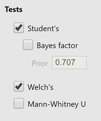
Go back to the options on the t-test dialog. There were the options under Tests. Select "Welch's" which will add a version of the t-test that does not require equal variances and corrects for unequal variances.
Now look back at the t-test output where the results of the t-tests are shown.
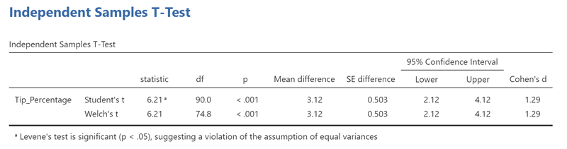
See how there are two rows of results presented, the top labeled "Student's tand the bottom labeled "Welch's t"? Well, if Levene’s test gives you a p-value less than .05, you use the bottom row because it does not assume that variances are equal. In fact, I would recommend using the bottom row all the time, just to be safe. The only thing you need to say when you use that row is that you are using a "Welch’s t-test".
Significance Testing
The test statistic, t, is reported under the column with the label "statistic": 6.21. To the right of it is another column you will need to report: "df", which stands for "degrees of freedom". For the bottom row, this number is not an integer: 74.838. To the right of it is "p", which is the p-value. It says "<..001".
The p-value indicates that a t value equal to or more extreme than 6.21 occurs less than 1 out of a thousand times (.001 = 1/1000) under the null distribution (assuming no difference between the two groups). This means that it is highly unlikely that the two groups are equal.
Under "Mean Difference", the t-test output adds a calculation of the difference between the means of the two groups: 3.12. You could calculate that yourself by comparing the means of the two groups: 17.74 vs. 14.62.
What is a Confidence Interval?
The last two columns present the "95% Confidence Interval". A confidence interval is a way of representing the precision of an estimate. In this case, the estimate is of the difference between the means of the two groups: 3.12. The confidence interval lower bound is 2.12 and its upper bound is 4.12, so it is plus or minus 1.0. A 95% confidence interval means that 95% of the time, the population mean will be within that interval and 5% of the time, the population mean will be outside of that interval. This means you can be 95% confident that the population mean is within your confidence interval.
What is the population mean? It is the value you would get if you could sample every member of the population in that condition. An important assumption with estimating a confidence interval is that your sample is representative of your target population. In other words, confidence intervals assume that if you collected more data, the new data would look pretty much like the data you have already collected: it would have the same mean and standard deviation.
In this case, the confidence interval is 2.12 to 4.12. You can be 95% confident that the difference between the population means for the Chocolate and No Chocolate conditions is somewhere between 2.12 and 4.12. As before, the confidence interval allows you to know the precision of your estimate. Serving customers chocolate with their check will increase your tip percentage somewhere between 2.12 and 4.12 percent.APA Style
To write up the results of this analysis, you could write:
Researchers hypothesized that giving customers chocolate with their bill would increase the tips that waiters received. Tip percentages for the two groups differed significantly according to Welch’s t-test, t(74.84) = 6.2, p < .001. On average, customers given chocolate tipped 17.7 percent, while customers not given chocolate tipped 14.6 percent. The 95% confidence interval for the effect of chocolate on tip percentage is between 2.1 and 4.1 percent. These results support the researchers’ hypothesis.
Common Error!
Note the formatting for reporting the results of the t-test:
- Write in complete sentences.
- State the researchers’ hypothesis.
- Give the means of each group, using the units for the dependent variable (here, the units are percentages because the DV was recorded in terms of tip percentages).
- Give the degrees of freedom in parentheses after the letter t (which is italicized)
- Give the p-value.
- Report the confidence interval.
- Decimal places: Use a number of decimal places sufficient to distinguish two values but generally not more than 2 or 3.
- State whether the results supported, partially supported, or did not support the researchers’ hypothesis.
Negative t values and confidence intervals?
The sign of the t-value is determined by whether the first mean is larger than the second (in which case, t is positive) or whether the second mean is larger than the first (in which case, t is negative). For example,if the no chocolate condition was listed first in your data file, you would be subtracting the mean of the chocolate condition from the mean of the no chocolate condition. Because chocolate had a higher mean, you would get a negative t score:
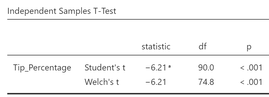
What if the confidence intervals are negative? If the t value is negative, then the confidence intervals will also contain negative numbers. So long as the confidence interval does not cross zero (does not contain one positive and one negative number), it will be much easier to interpret it if you use the absolute value of the confidence interval. So, if the confidence interval is between -4.1 and -2.1, you would rewrite it to say that it is between 2.1 and 4.1 (in ascending order) . So just drop the negatives in your report.
95% Confidence Intervals Crossing Zero
There is an interesting relationship between confidence intervals and the p-value for t-tests. If a 95% confidence interval of the difference between means crosses zero, then the t-test of that comparison will not be significant at p < .05. So, if you find that the confidence interval of the difference between means is -3.2 to 7.5 points, you know that the p-value of the t-test will not be significant at p < .05 because -3.2 to 7.5 crosses zero. If a confidence interval of a difference crosses zero, it means that the difference could be zero, and that means there could be no difference at all.
So, you now know how to use a boxplot to check the distribution of your data and how to use an independent t-test to test whether the means of two groups are significantly different. One step remains: How to create a plot that shows the means and confidence intervals. That is the topic of the last page.