Plotting Means and Confidence Intervals
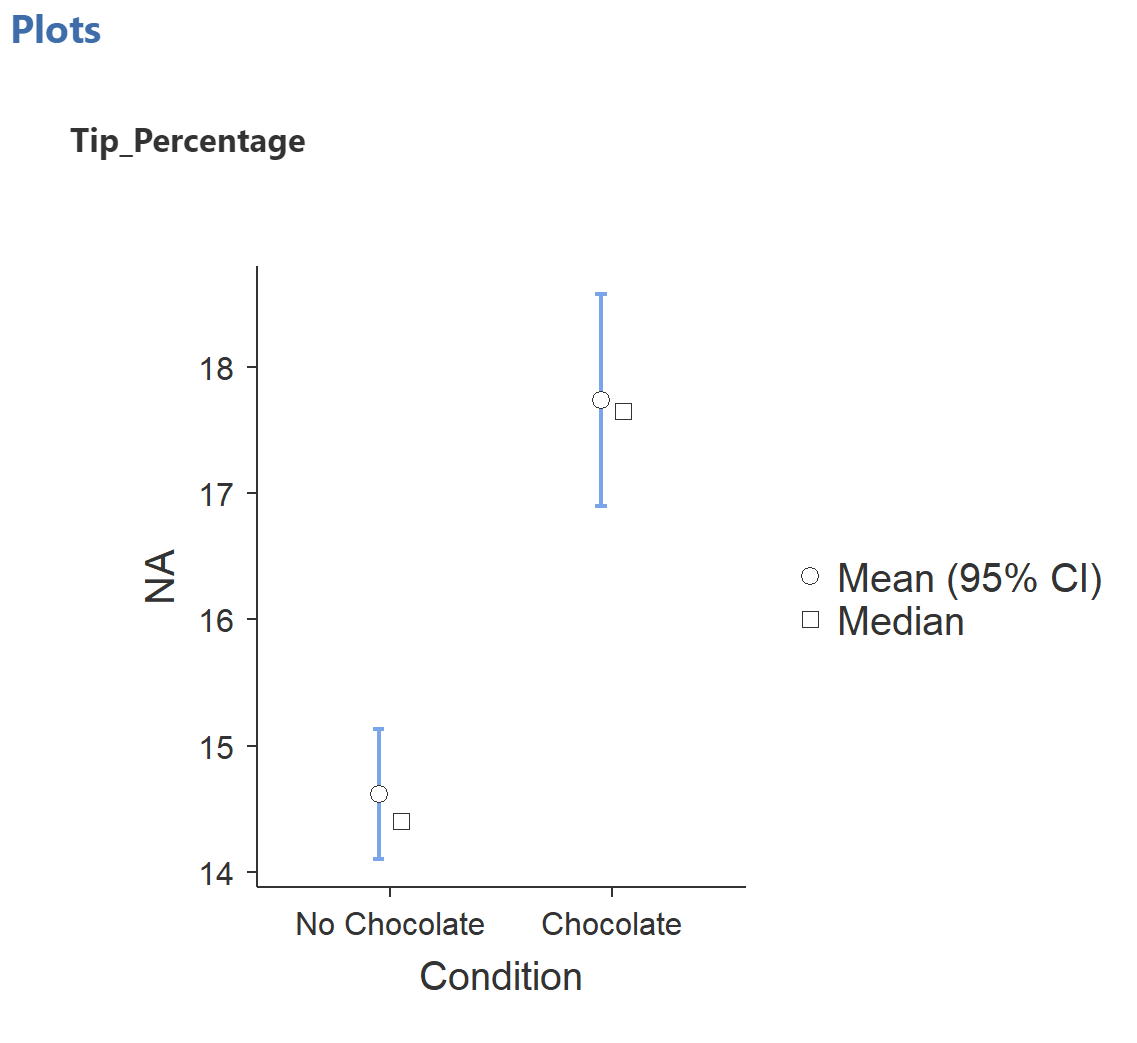
Boxplots are very useful for examining the distribution of your data, but if you are using a t-test to compare means, boxplots are somewhat misleading because they show the median instead of the mean, which is what the t-test uses. There is a different plot which popped up whe you slected "Plots" under Additional Statistics": Go to the output window and scroll down. You should see somethink like below.
Changing to Excel to be able to adjust the graph.
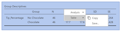
Currently in Jamovi, you cannot adjust the plot, but you can copy the descriptives from jamovi.Right click on the describes table. You should see the following menu pop up:
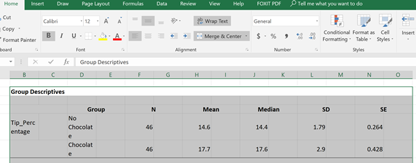
Select "Copy" and go to Excel and paste the data in a convenient cell. You might need to increase the font size, just go to the home ribbon and change the number next to the font name ("Calibri") in the example below.
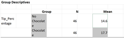
To make the chart creation easier in Excel, first click in any empty sell to clear your paste selection. Then clcik on the two cells below "Group" to get the names of the two conditions. Then, Control-click (command-click for Macintosh) the two cells below mean. We have to control click because the cells are not right next to each other. You should have something that looks like:
Choose the Insert Ribbon and select Recommended Charts and it will have as a first option (In Macintosh, it might work easier to go to the Column Chart and select "Clustered Column" chart). You should see an dialog box likc below:
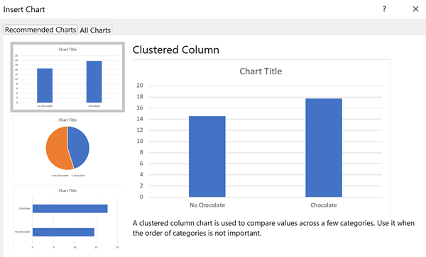
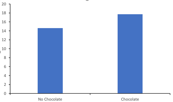
We will chose what Excel calls "Clustered Column" which should be the first choice. Of course, every other person calls this a bar graph. Oh well. When you select this chart, you should see something like I show below.
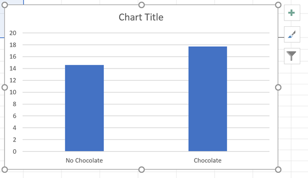
Unfortunately, this graph will not do. Excel does not understand the expectations of a good graph in psychology or eve APA format expectations. So we have some work to do. But the strength of Excel is how much you can modify a graph.
First, select by clicking on Chart Title and then press "Delete." Do the same with the horizontal lines which are more distraction than worth. Click on any one of them go select and then press "delete." The graph should not look like:
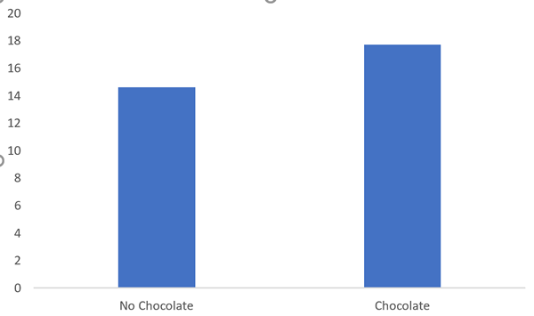
First thing we have to do is put on axis lines. Right click on each, one at a time, axis and select "Format Axis" on the pop up menu. You will see a dialog box open on the right. Select the titled paint can symbol and you will see something like this:
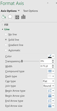
If you need to click on the triangle next to "Line" to open the options. Make sure you select "Solid Line" and change the "Color" to black for the axis. When you have done both axes you should see this:
Click on the graph and notice the plus sing on the upper right corner. Click on it and you should a menu open up a lot more clearly than what is shown below.
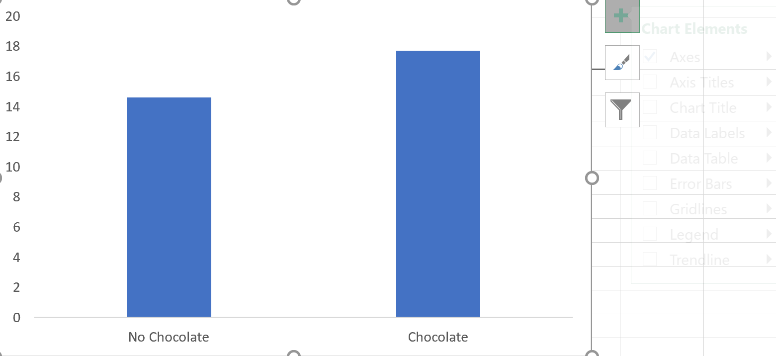
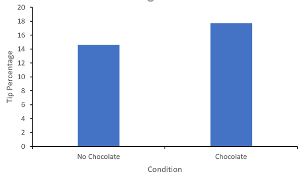
You bring up the option menu for each feature of the graph by clicking on the triangles on the right. Now, add axis titles selecting both the "Primary Horizontal" and "Primary Vertical" axis. After slecting each axis title option, just start typing and then hit enter. For the "Primary Horizontal" axis, put in "Condition" (without the quotation marks) and for the "Primary Veritical" axis, enter "Tip Percentage". You should have below.
Adding Error Bars
It is of paramount importance to indicate both the mean and the variation of the data. We do this by added error bars around the mean. There are many choices for error bars, but we are going to use 95% confidence intervals. To plot these we need to go back to the spreadsheed in Excel and do one small computation.
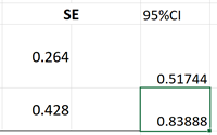
Go back to the data in your spreadsheet and look for the column called "SE" (for standard error). You might need to drag the graph out of the way. Recall that the standard error is the standard deviation fo the sampling distribution of the mean. We need to adjust it so that we will have 95% of the sampling distribution of the mean in the error bars. So we need to multiply the standard error by 1.96. In Excel, in a cell to the right of the "SE" and type "=1.96*" and then click on the box with the top standard error. You should see something like:
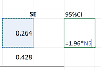
HIt enter. Then copy and past that cell below and you should see:
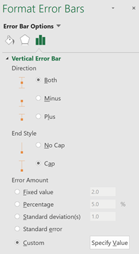
We will used these value for our error bars.Return to the graph and select the plus in the upper right corner of the chart and select "More options". A dialog box shoulw open. Select the icon of of three vertical bars and then at the bottom select "custom" Excel really has no idea about error bars so we have to go out of our way to put in meaningful one. The dialog box should not look like below:
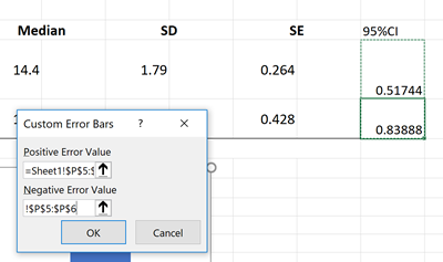
Select, "Specify Value". A dialog box will pop up with two small windows. At the end of each window, click on the the upward pointing arrow and then select the Confidence Interval values you just calculated. Yes, select the exact same cells to go into both windows.When you are done selecting the cells, it should look something like this:
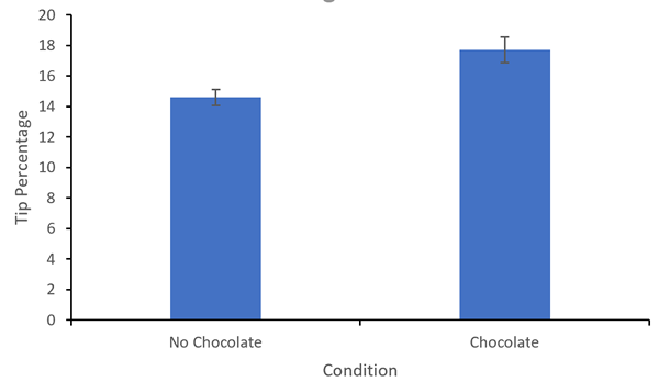
Select "OK" and you should now have a final graph that looks like:
Smaller Samples Mean Bigger Confidence Intervals
The confidence intervals you have generated are based on 92 data points, 46 in each group, and they are fairly narrow. That's good because it means that you have a more precise estimate. To see how confidence intervals get bigger as sample size decreases, look at the two plots below.
First is the original plot, with all 92 subjects, and second is a plot made from a random sample of 30 of those subjects.
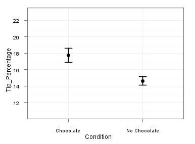
92 subjects
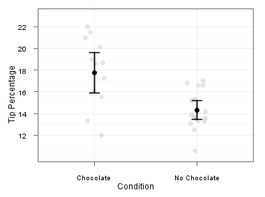
30 subjects
Note how the confidence intervals in the first plot are smaller than the ones in the second plot. With more data, your estimate of the means is more precise. In the second figure, you can be 95% confident that the population mean in the Chocolate condition is somewhere between a 16 and 20 percent tip. In the figure on the left, that interval shrinks to a 17-to-19 percent tip. Your estimate of the mean has become more precise.
A Note On Bar Graphs
The choice of the graph is very important in communicating accurately what is going on in your results. Bar graphs should be choisen very carefully. We will develop over the term skills in selecting the appropriate graph format. Why can we use a bargraph here? First, on the x-axis we have a nominal variable. Bar graphs are good here becase they do not connect the data along the x-axis. But also important, we have a ratio variable, tip percentage, on the y-axis and as such we have an absolute 0. That 0 value is plotted on the axis. When using bar graphs, it is important that the y-axis range is ratio and that the 0 is plotted. Otherwise we will still see the y-axis as ratio and still look at the data in this way visuall making a ratio of the bars. I would recommend avoiding a bar graph unless these conditions apply.
Homework
There is a stats homework assignment on comparing means (and reviewing reliability) that accompanies this tutorial. To begin the assignment, you can log in to your moodle account for this course.