Size Constancy Lab
II
Background:
- Purpose and Goals
- To determine the depth cues that provide the best
size constancy.
- The develop an understanding of the difference
between quantitative and qualitative predictions
- To compare data to hypothesis when the hypothesis
is mathematically precise
- To learn more about designing your own experiment
- Size Constancy - Briefly, will discuss more in class
next week of classes
- Recall from class
- This week we will add a Monocular Cue
- Quantitative Predictions
- A qualitative prediction deals with trends.
- An example would be from the retinal acuity
lab
- acuity gets worse farther out in the
periphery.
- This statement does not predict how
worse. Thus, it is qualitative.
- A quantitative prediction deals with both trends,
but the size of the trends.
- To apply this to the last lab it might say,
for each degree of visual angle out from the
fovea acuity gets worse by 10%.
- This type of statement allows a much finer
test of the idea.
- This type of statement can also be written as
an equation
Acuity = (distance from Fovea * .10*acuity at
fovea)+
acuity at fovea.
This is simply a translation of the statement
at 3.b.i into a mathematical expression.
- Quantitative Elements of this situation.
- Size Constancy
Sr
α 1/dp
Sp
= k
Sr is the
size of the retinal image
Sp is the
perceived size of the object
dp is the
perceived distance of the object (since in
our case the distances will all be
virtually created)
α means proportional to.
k is a constant.
To translate all this into English: The
retinal image size decrease as distance
increases such that they are
proportional. That means as distances
doubles, the height of the image in the eye is
cut in half. However, the perceive size
stays the same regardless of the change in
image distance.
- Perceived Distance
Distance from Screen = Viewing dist(mm) *
disp(mm)
Interpup dist (mm)
Perceived Dist = Viewing Dist - Dist from
Screen
- These will be brought together when the
experiment is explained
The Experiment:
- Equipment
- Here is the link to the lab experiment: ISLE 7.4 (b.2) Size Constancy
Experiment
- Design:
- Arrangement of Stimuli:
Standard
Comparison
- IV1 is amount of depth (in this case, amount of
binocular disparity).
- IV2 is the depth cue being tested:
- Today we are adding texture gradient
- Next week we add relative height
- DV is size of comparison circle relative to the
Standard (left) circle
- Method:
- Viewing Distance is 75 centimeters (be precise and
convert to millimeters for the calculations below).
-
Open the lab webpage.
- Stimulus Settings:
- Select texture gradient and disparity
- Chose the depth setting for your monocular
cue.
- Chose the same number of levels for depth as
week 1 for steropsis but fill the possible
range
- Make sure the relative settings for the two
depth cues are the same
- Note that they use different number ranges
- Fill the range of texture gradient.
- Measure how the screen looks for all of your
settings
- These number values are mostly convenient to
the program and nothing real
- Make sure all other depth cues are unchecked
this week, except disparity
- So when setting each condition yiou will
set two depth settings: A disparity setting
from last lab and a matching texture
gradient setting
- Next week we will add relative height.
- Method Settings: Method of Adjustment
- We are Measuring a Point of Subject Equality
(PSE). What is this?
- Choose Number of Trials: Should do several
(USE THE SAME AS LAST WEEK FOR THE METHOD)
- Set the parameters for the method as you
think will give you sufficient data and
clean results
- Again, try some of the settings out
- Messy results may be easy to collect but
no fun to interpret
- Leave range of variation and maximum and
minimum values unchanged
- Procedure:
- On each trial respond as directed on the screen.
- Generating Predictions:
- First, make sure all measurements are in the same
units, i.e., millimeters, or your answers will be
incorrect
- The two measurements you need off of the screen
are the size of the standard (left) circle and the
disparity
- These measures are illustrated below
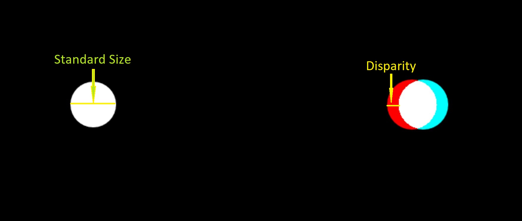
- To measure the standard size, measure the
diameter of the left hand circle
- To measure disparity, measure, for each
disparity setting, the distance from the edge of
one color to the edge of the white where the two
colors overlap
- If you use the same setting for crossed,
positive, and uncrossed, negative, disparities,
you only need to measure the disparity once. Use
either the crossed or the uncrosse disparity
- Keep the sign on your disparity. If you are
measuring a crossed disparity, keep your
measurement positive. If you are measuring an
uncrossed disparity, put a negative sign in front
of your measurement
- Measure Perceived Distance for each disparity
condition: e.g., viewing distance = 750 mm,
disparity = 3.4 mm, interpupillary distance = 63 mm
- Distance from Screen = (750mm * 3.4mm)/63mm =
40.5 mm
- Perceived Distance = 750mm-40.5mm = 709.5mm
- According to Size Constancy: when two objects
appear the same size the retinal image sizes are
inversely proportional to the two distance.
- in English, an object that is twice as far
away has to be half as tall on the retina to
appear the same size. To do this for this lab,
divide the distance from the screen by the
perceived distance since the depth is virtual,
we are dealing with Emmert's Law
- So, the predicted relative size is
750mm/709.5mm = 1.06 (note, no units as the two
mm cancel each other out)
- Write-up: (Full report)
- Week 3: Do a graph of your predictions for the
stereopsis condition to hand in so I can inspect
them
- Type of graph is an x-y (scatter), using Excel's
term
- The x-axis should be your disparity, in the
millimeters you have measured off of the screen,
not the settings from ISLE
- The y-axis is your predicted relative size (no
units)
- At end of lab, do all sections of the lab report
specified in the lab
report format. This will be due two weeks
after lab.
- This lab report has a particularly complicated
stimulus section you need to measure the
following elements:
- The disparity in mm: from edge or color
(red or cyan) to edge of white on same side
- The size of the standard in mm
- Will talk more measurements later
|
|