Correlation
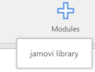
Correlation is a statistical procedure designed to measure the strength and direction of the linear relation between two variables. As values on one variable increase, do values on the second variable tend to also go up? Go down? Do nothing? On this page, we will be working on how to plot correlational data. On the next page, we will discuss how to use statistics to assess correlation. To do this activity, we will learn a new feature of Jamovi. There are plug ins you can add, called Modules. Click on Modules and then Jamovi LIbrary that shows up when Modules is clicked.
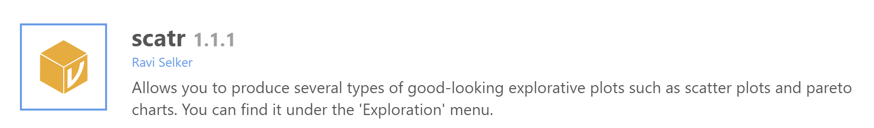
In the window that pops up, scroll down the modules and select SCATR and press the Install button right below it.
Data for Example: Chivalry Questionnaire
For this exercise, you’ll be working with some questionnaire data from 411 students. You can access the data in the following Excel file:
The questionnaire included five measures of gender role attitudes:
- Chivalry (chiv), a measure of the degree to which a person endorses the idea that men have more of an obligation to protect and provide for women than vice-versa.
- Moral Virtue (MVIRT), a measure of the degree to which a person believes women are more morally virtuous (have a better conscience, more morally "pure," etc.) than men.
- Sexual Virtue (SVIRT), a measure of the degree to which a person believes that women are more sexually virtuous (think about sex less often, don’t think about others in sexual ways, etc.) than men.
- Attitudes toward Women Scale (AWS), a published measure of conservative or traditional gender role attitudes (e.g., women should not work outside the home). This measure was obtained for only half of the sample.
- Female Agency (agency), a measure of the degree to which a person believes that women are as competent and as well-suited to positions of authority as men are.
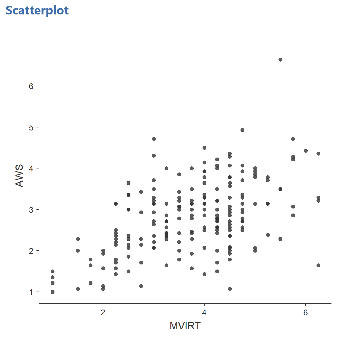
Step 1: Plot Your Data!
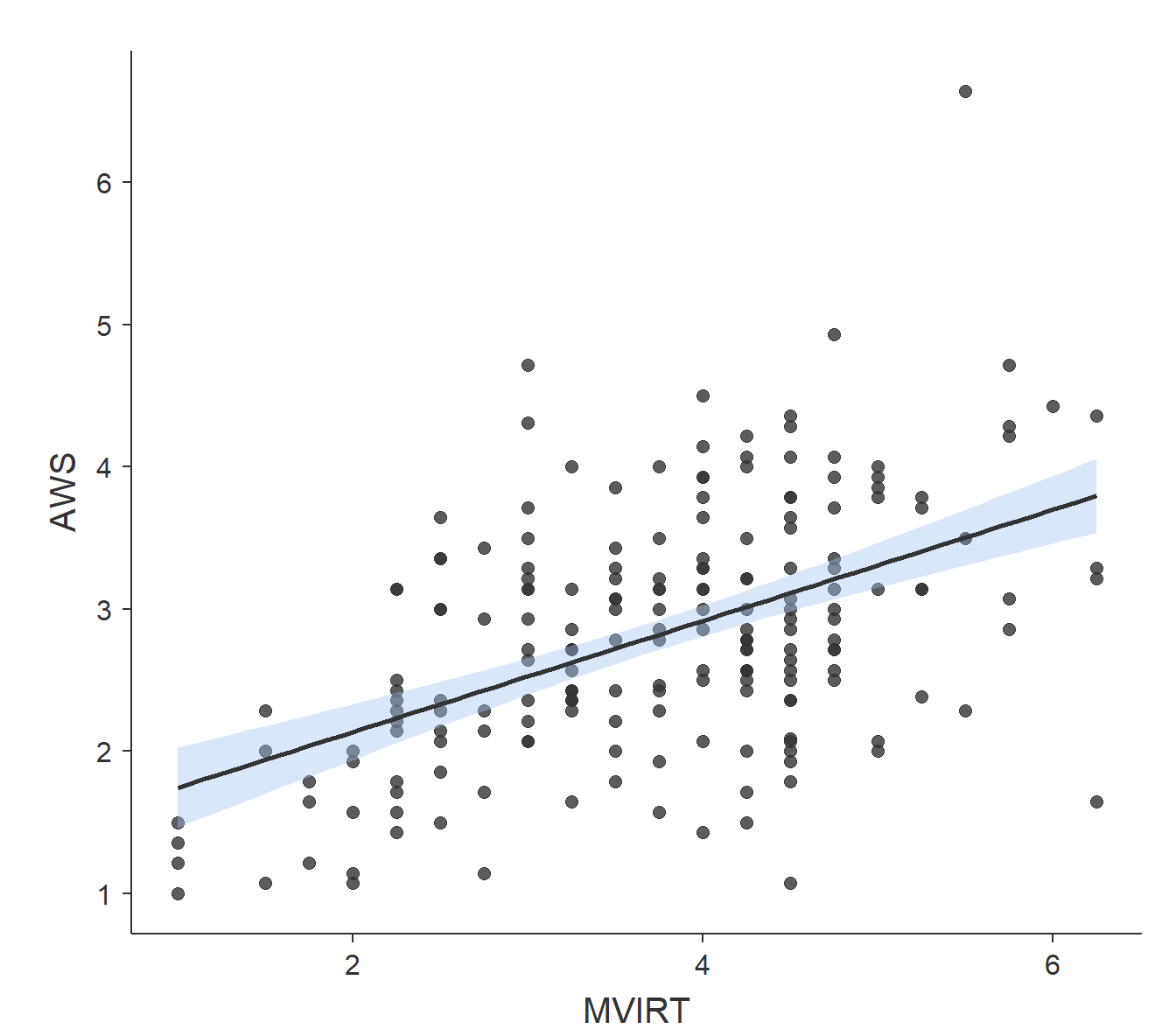
The plot above is called a scatterplot. Each point in that plot refers to two measures of a single observation. In this case, each point refers to the AWS and MVIRT scores of a single person. As you can see, low scores on AWS tend to be found with low scores on MVIRT, while high scores on AWS tend to be found with high scores on MVIRT.
Scatterplot in Exploration
To get this scatterplot, select Exploration → Scatter Plot. In the scatter plot dialog, put AWS on the x-axis and MVIRT on the y-axis. You should get this:
Adding a line of best fit
In the first scatterplot (with the white background), there is a solid line with a blue area around it going through the data. The center line is the line of best fit, a line that minimizes the vertical distances between the data points and the line itself. The “best fit line” is a useful way of representing the linear trend in a scatterplot. It helps capture the pattern indicated by r = +0.5: higher scores on AWS are found with higher scores on MVIRT. The blue area around the center line represent the upper and lower bounds of the 95% confidence interval around the line of best fit. You can have 95% confidence that the line of best fit for the population (the “true” best fit line) is within the confidence interval. Note that the confidence interval is not reflective of where 95% of the data points are. It corresponds to where the line of best fit would be drawn, not to where data are likely to appear.
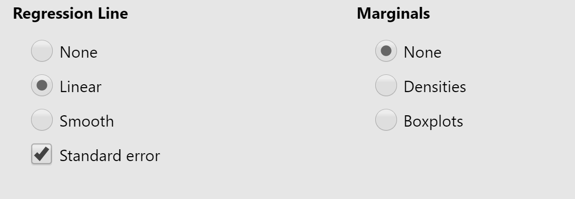
To add a best-fit line to your plot, below the box with the variables under Regression Line, select Linear and Standard Error as seen below.: