Two-way ANOVA
Frequently, you will want to examine the effects of more than one independent variable on a dependent variable. When your design includes more than one independent variable, it is called a factorial design.
Consider a study by Johnson and Rusbult (1989, Experiment 2) in which they investigated the tendency for people to "devalue unselected alternatives." For example, when a student selects college A over college B, she will tend to devalue college B (see it as worse than before) as a way of justifying her decision. Johnson and Rusbult investigated this phenomenon in romantic relationships. They expected that single people would anticipate more happiness with a very attractive prospective partner than with a prospective partner who was only moderately attractive. Their second prediction was that people in a committed relationship would not show this pattern. Like the student attending college A, people in a committed relationship have made their choice and will devalue the unselected alternative, who in this case is a very-attractive prospective romantic partner. Thus, the researchers are predicting an interaction: the simple effect of attractiveness will be stronger for single participants than for committed participants.
I constructed a simulated dataset based on Johnson and Rusbult’s study, which you can access here:
The JR89E2 dataset has 3 variables:
- Commitment: a factor set to either “Low” or “High”, indicating whether the subject was in a committed relationship.
- Attractiveness: attractiveness of target prospective romantic partner, either “Low” or “High”
- rating: average of several ratings. Higher scores indicate more attraction to the prospective partner.
Step 1: Statistical analysis
Overview
When you analyze a factorial design, you are testing for the main effect of each of your independent variables as well as the interaction between those independent variables. In this case, you are testing for the main effect of Commitment (whether ratings of the target differed based on the subjects’ level of commitment to their current relationship, ignoring the effects of target attractiveness), the main effect of Attractiveness (whether ratings of the target differed based on the target’s attractiveness, ignoring the effects of subjects’ commitment to their current relationship), and the interaction between Commitment and Attractiveness (whether the effects of one factor are different depending on the level of the other factor).
General Linear Model: Univariate
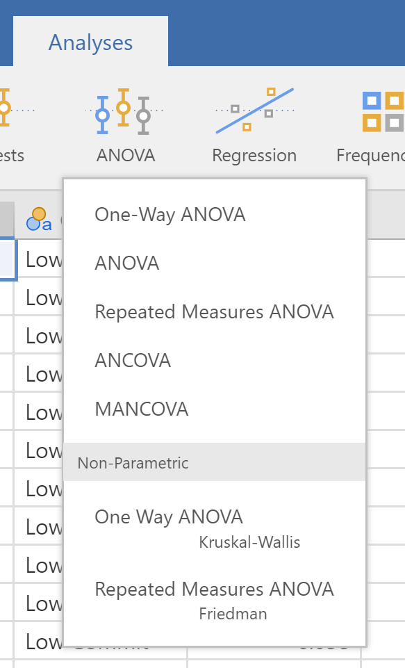
To get started, select ANOVA → ANOVA.
Put “rating” into the “Dependent Variable” box. Put "Commitment" and “Attractiveness” into the “Fixed Factors” box.
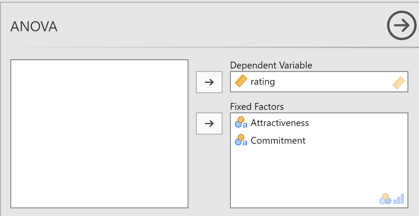
A factor is the term Anova uses because the study might be an experiment which an independent variable or a correlational design when what you have are groups, especially one that is nominal-scale (categorical). A fixed factor is a factor that takes on only a small number of values that represent levels that the researcher is interested in comparing.
Setting up tests of simple effects
Before you click OK, click on the Options button. We need to set things up so that the output will include tests of the simple effects. Put “Attractiveness” in the “Display Means For” box, checkmark the “Compare main effects” option, and set the “Confidence interval adjustment” to Bonferroni.
ANOVA Output
In the window to the right, we see an ANOVA table:
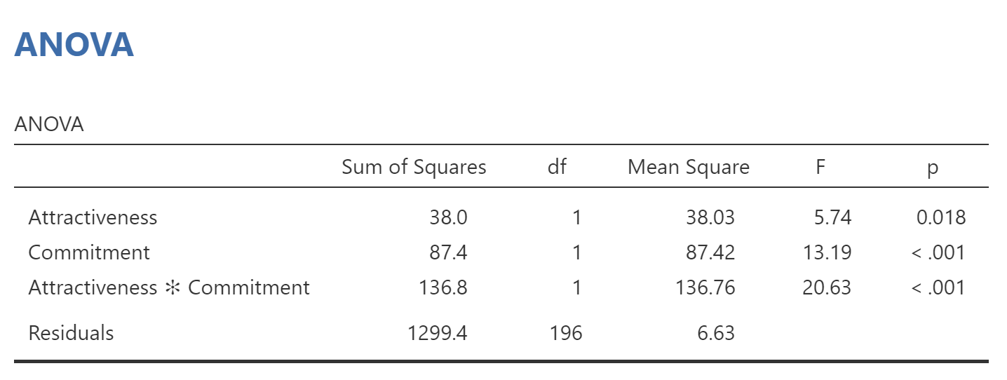
The first two rows show us the tests for the main effect of attractiveness, the main effect of commitment. The third row shows interaction between attractiveness and commitment (“Attractiveness * Commitment”). The “p.” column tells us that all three effects are significant at p < .05. Here’s how we could summarize the results of that table in APA style:
Partner ratings were analyzed with a 2 (Attractiveness: Low versus High) x 2 (Commitment: Low versus High) between-subjects ANOVA. The main effect of attractiveness on partner ratings was significant, F(1,196) = 5.74, p = .018. The main effect of commitment on partner ratings was also significant, F(1,196) = 13.19, p <.001. There was a significant interaction between attractiveness and commitment, F(1,196) = 20.63, p < .001.
Some notes on the results printed above:
- When you report a main effect or an interaction, the test statistic is an F. It is reported with two “degrees of freedom” (df). Those are the two numbers inside parentheses given after the “F”. The first df is from the row for the effect in question. It is equal to the number of levels of that independent variable, minus one. Because there are two levels of each independent variable, df is 1 in each case. The second df is the degrees of freedom for the row labeled “Error”. In this case, that number is 196. That is why each of the F statistics above starts out “F(1,196)”.
- Given any F-value and 2 degrees of freedom, it is possible to compute its p-value: the probability of obtaining that F-value just by chance. If the p-value is below your alpha level (the threshold you set to call something “significant”, usually .05 in psychology), then you say the main effect or interaction is “significant”. In the table above, each p-value is less than .05, so each of the effects is identified as “significant”.
One problem with the APA-style description given above is that it only tells us that there were significant effects, but it doesn’t tell us the pattern of those effects. To get that information, we need to look at the plot and the results of the pairwise comparisons. We’ll do that on the next page.